Generic pipeline for EEG-fMRI processing: Example on fingertapping experiment

Author: Hadi Zaaiti <hadi.zaatiti@nyu.edu>, Puti Wen <puti.wen@nyu.edu>

In this notebook we will process EEG-fMRI data from a fingertapping experiment and provide the pipeline to be adapted to your own experiment.

Different modalities for processing EEG-fMRI data exists in the literature:

• assymetrical approach where one modality (EEG or fMRI) constrains the other modality

  • mainly the EEG data constrains temporally the fMRI data

  • or the fMRI data constrains spatially the EEG data

• symetrical approach where both modalities constrain each other

The assymetrical approach seems more popular in the literature.

Required Data

• fMRI data consists of

  • times series of Bold signals mapped to a geometric space (either to each voxel, or to vertices of a surface)

  • at NYUAD, an fMRI dataset consists of multiple files in dicom format

• EEG data consists of

  • A .eeg file: raw data from the electrodes (time series)

  • A .vhdr or .xhdr file: a header containing metadata on parameters and sensors, layout of coordinates of sensors

  • A .xmrk file: contains markers with their time (can be opened in a text file)

• for source reconstruction

  • EEG/FMRI requires a T1 image (the subject should not have the EEG cap while getting the T1)

Example of such datasets are present on NYU-BOX. Demo dataset of finger-tapping has been provided and are available on the recording computer:

The generic pipeline for EEG-fMRI data processing involves the following steps, detailed below

References

1. Cilia Jaeger (2024). BP Academy Webinar Recording: Combined EEG and fMRI data analysis.

   • Youtube webinar available at https://www.youtube.com/watch?v=vGQVeCn53ys

   • EEG-fMRI Data preprocessing and considerations - Session 2: https://youtu.be/5EqyURlZDMA?feature=shared

   • Combining EEG and fMRI data analysis – Session 3: https://youtu.be/vGQVeCn53ys?feature=shared

Preprocessing of the EEG data

Preprocessing of the EEG data involves multiple step. We will be using BrainVision Analyzer. Plug the BrainVision dongle onto any windows comptuer you will be using it for the Analysis.

• Open BrainVision Analyzer

• Create three folders in a directory, name them as follow

  • export: this will contain exported data from analysis pipeline

  • history: this will contain all processing steps

  • raw: put your raw .eeg, .vhdr, .vmrk here

EEG data triggers

The EEG data from an EEG/fMRI experiment should have the following trigger signals

• Sync On of marker type Sync Status is a marker repeated every period of time ensuring that the MRI clock and EEG system are in sync

• T 1_off of marker type Toggle is a marker

  

  One TR (repetition time) corresponds to T 1_off - T 1_on.

ECG Removal

• The subtraction method can work better than ICA, use the substraction method to remove ECG signals

Steps for noise removal and pre-processing

• Gradient artifact correction:

  • Always remove the gradient artifacts first.

  • ECG with gradient artifacts can be saturated sometimes, which means that the ECG sensor should be moved around.

  • MRI artifact correction: then pick use markers, then R128, making sure the correction is only during these triggers and not for the rest.

  • Then Next.

  • Artifact Type is always Continuous (interleaved was an old thing when MRI was collected for a period of time and then EEG for another period of time).

  • Enable Baseline correction for average (compute baseline over the whole artifact).

  • Use sliding average calculation to account for changes in gradient artifacts over time.

  • Do not select Common use of all channels for bad intervals and correlation.

  • Then next: select all EEG channels (only time we don’t use all channels is if we are measuring a specific thing).

  • Then next: deselect downsampling (we can do this later).

  • How to store data Select store corrected data in a cached file.

• ECG signals correction after gradient artifact cleaning:

  • Also use a sliding average subtraction approach (Not ICA), use ICA if there is a residual.

  • We do not have markers on the peaks (this is needed for the subtraction method).

  • We need to add R peaks (peaks on the ECG signals).

  • After the gradient artifact correction, some high-frequency noise stays in the ECG channel during MRI acquisition.

  • Apply High Cutoff Frequency: go to Transformations, then IIR filter, disable the Low cutoff and High cutoff of all channels, then select only the ECG channel and apply a high cutoff (15 Hz), then apply filter.

  • Then Transformations, Special Signal Processing, then CB correction.

  • Choose the ECG channel (if it’s a clear heartbeat, if not use another EEG channel that shows a clearer one than ECG).

  • Go through the manual check if the automatic analyzer skipped some R peaks.

  • After selecting all the R peaks (which should be marked in Green), click Finish.

  • Then the R peaks should appear on the peaks as R.

  • Go to Special Signal Processing, select CB, then select Use Markers, then select R markers.

  • Then next, and use the whole data to compute the time delay. The total number of pulses is the sliding signal window. Empirically, we use 21 as the parameters.

  • Select all EEG channels except for CWL and the ECG channel.

• Carbon Wired Loops (CWL), accounts for movement correction:

  • Change sampling rate: we need to downsample and then apply the CWL regression.

We can automate the process by saving all the analysis steps.

Helium Pump Noise:

• Components around the 50Hz frequency should appear in all channels.

• The helium pumps cannot be turned off during an experiment.

Pre-processing steps should involve:

1. Inspecting the static field data.

2. Gradient-artifact correction.

3. ECG correction or CWL regression (Cardioballistic artifacts).

4. Classic EEG analysis.

Pre-processing of the fMRI data

Figure 1: Overview of the fMRI Pre-processing Steps (Red: Run on XNAT, Blue: Run Locally)

Overview

The MRI scanner at NYUAD provides the data in dicom format stored securely on an XNAT platform hosted on NYUAD servers.

• We store and organize raw scanner data in XNAT.

• We convert these data to BIDS format using dcm2bids.

• We perform standardized preprocessing with fMRIPrep.

• We rely on NYU Box, Jubail HPC, and XNAT for secure data transfer, computation, and storage.

Together, these tools produce reproducible, GLM-ready fMRI outputs.

Converting DICOM to BIDS on XNAT (Not tested)

• Prerequisites for Running dcm2bids

  1. Ensure your DICOM data are properly uploaded to your xnat project.

  2. Confirm you have an active xnat account with the necessary access permissions.

• Running dcm2bids

  1. Navigate to your xnat project.

  2. Prepare a dcm2bids configuration JSON file containing all required scan-to-BIDS mappings, and store it on xnat.

     • example config file for the finger-tapping experiment can be found in pipeline/eeg_fmri_pipelines/fmri_preprocessingutilities together with a batch script to help run dicom2bids command

     • Click on your project, then Manage Files, select resources for level then add Folder called configs then upload file config.json

  3. Select the Processing Dashboard, and then MR Sessions

     

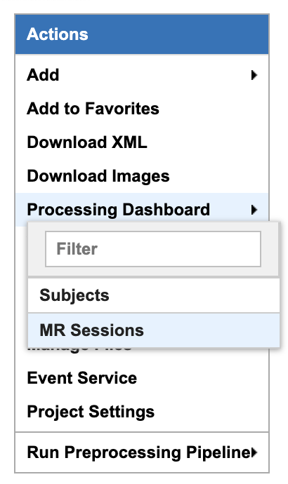
  4. Under Select elements to launch processing, in dropdown menu Select Job, select dcm2bids-session

  5. Select Subjects you want to process, and click Launch job

  6. Click Reload to see the job status and wait for it to finish (this may take a 5-15 minutes)

  7. Sanity check after running dcm2bids

     • After running dicom2bids, we want to verify the file structure:

       1. Ensure the expected folders are present: - Func/ - Eeg/ - Anat/ - Fmap/

       2. Check filenames and parameters.

     • Ideally, each task has its own sbref (two files: one AP, one PA)

     • Similarly, fmap should have AP and PA (not for every run, but for every task)

Converting DICOM to BIDS on local computer (tested)

• Install dicom2bids and dicom2niix

• Download your session from XNAT

• Adapt the config.json to your project

• Ensure an anatomical T1 is in your DICOM directory

• Run dicom2bids_config_script.bat to generate the BIDS output

  • Customize the batch script to put the correct subject ID and XNAT downloaded directory

• There is another script for the T1 if added later on

• Run post_conversion.bat (this will replicate SBref AP and PA for each bold run)

  • Customize the batch script to provide your BIDS output directory

• Run BIDS validator online on your BIDS directory to make sure there are no errors

• In the output .json in the bids directory, open the .json for the fmaps and delete the bids:: in the “IntendedFor” field

fMRI Preprocessing with fMRIPrep: Two Available Routes

• Route 1 (Red Path): Running fMRIPrep on XNAT (Not tested)

  1. Running fMRIPrep on XNAT

     • In dropdown menu Select Job, select bids-fmriprep-session-jubail

     • Select the Subjects you want to process, and click Launch job

     • Click Reload to see the job status and wait for it to finish (this may take a 4-8 hrs)

  2. Returning fMRIPrep outputs from XNATto NYU BOX

• Route 2 (Blue Path): Running fMRIPrep Locally (tested)

  1. Downloading data from XNAT to Jubail

  2. Running fMRIPrep on Jubail

     1. Download the fMRIPrep image on Jubail

     2. Prepare the sbatch script

     3. Submit the sbatch script

  3. Returning fMRIPrep outputs to NYU BOX

     rsync -av [YourNetID]@jubail.abudhabi.nyu.edu:/scratch/MRI/[YourProjectName]/ /local/path/to/NYUBOX/[YourProjectName]/
     

Route 2 fMRIPrep locally (on HPC Jubail)

Once the BIDS directory is created then you can install fMRIprep on jubail, copy your BIDS data directory to Jubail then process your data.

• Copy your BIDS directory to /scratch/username/MRI/Project_name/

Two scripts can be found under pipeline/eeg_fmri_pipelines/fmri_preprocessing/utilities: - get_fmriprep_image.sh run this script to pull the fMRIprep image and extract it - The following command will place the fmriprep image into the /scratch/username/mysif/ folder

sbatch get_fmripre_image.sh

• Download templateFlow (required to register data into template space)

  • module load NYUAD/4.0

  • module singularity/3.8.0

  • module braimcore/3.1

  • run the following commands

    export BRAIMCORE_ENGINE=fmriprep
    braimcore fetch_templates
    

  • Get a free surfer license from https://surfer.nmr.mgh.harvard.edu/registration.html

• Examine the run_fmriprep.sh script, ensure that your username is correct and set the other parameters relative to your project, the provided example is for the finger-tapping experiment

• You can now run fmriprep using the following:

  sbatch run_fmriprep.sh
  

• Monitor the job and the logfiles for a short amount of time

  • You can see the error logs as specified in the header of the run_fmriprep.sh script for the SLURM job

    • #SBATCH –output=/scratch/$USER/MRI/fingertapping/fmriprep_%A_%a.out

    • #SBATCH –error=/scratch/$USER/MRI/fingertapping/fmriprep_%A_%a.err

  • Monitor these logfile at the beginning of the launch to make sure the job has not encountered an early error and stopped

  • Use the ‘squeue’ command to see if the job is still running

  • To cancel a job scancel (JOB_ID)

  • If you are fixing an error and executing fmriprep again, make sure to first empty the derivatives directory (as leftover files from a previous run can leave incorrect data)

• After fmriprep has finished executing you will see in the derivatives folder the fmriprep output

• An example of the output html can be found here View fMRIprep output HTML

• Ensure that “Susceptibiliy distortion correction” has been correctly applied, this can be viewed from the output HTML

  • if this is not the case, it means probably that the “fmap” part is not configured correctly

  • From the output of dicom2bids, change the fmap .json file to remove the bids://

  • Change in the fmap directory, in the .json’s, in the Intended For field, change the slashes from // to \

At this stage, you now have successfully ran fmriprep and obtained a correct output bold signals that are corrected for distortion. The next step would be to learn GLM’s given the bold signals

Output spaces note

The --output-spaces argument in fMRIPrep specifies the spatial reference spaces in which preprocessed functional data will be output. You may combine multiple volume and surface spaces, and optionally control the resolution or surface mesh density.

–output-spaces T1w:res-native fsnative:den-41k MNI152NLin2009cAsym:res-native fsaverage:den-41k fsaverage

Example usage used in the run_fmriprep.sh script:

–output-spaces T1w:res-native fsnative:den-41k MNI152NLin2009cAsym:res-native fsaverage:den-41k fsaverage

Options explained:

• T1w:res-native

  Outputs the data in the subject’s own anatomical (T1-weighted) space, preserving the original resolution of the functional data.

• fsnative:den-41k

  Projects the data onto the subject’s native FreeSurfer surface (fsnative), with a mesh density of approximately 41,000 vertices per hemisphere.

• MNI152NLin2009cAsym:res-native

  Normalizes the data to the MNI152NLin2009cAsym standard volume space (asymmetric version of the 2009 MNI template) while maintaining the native functional resolution.

• fsaverage:den-41k

  Projects the data onto the standard FreeSurfer average surface (fsaverage) using a mesh density of ~41k vertices per hemisphere.

• fsaverage

  Projects data onto the default fsaverage surface resolution (~163,842 vertices per hemisphere). Including both fsaverage:den-41k and fsaverage may be redundant unless explicitly needed.

Note

The res-native flag is particularly useful when you wish to avoid unnecessary interpolation or smoothing that occurs during resampling.

For further details on available spaces and how they are handled, see the fMRIPrep documentation.

Learning Generalized Linear Models (GLM) from fMRI data

• Define the following environment variable in your .bashrc (to be seen by the terminal) and .profile (to be seen by MATLAB) by adding the following lines at the end of the files

  ..code-block::bash

  export BIDS_DIR=/mnt/rcs_mri/projects/MS_osama/hadiBIDS/fmriprep_output_from_HPC/derivatives export EEG_FMRI_DATA=/home/${USER}/Documents/EEG-FMRI export FREESURFER_HOME=/usr/local/freesurfer/8.0.0

• in the fmriprepoutputsub-0665func output directory you will find:

  • files ending in func.gii

  • files ending in func.mgh

  • files ending in nii.gz

• we had requested for 5 output spaces

  • each run will have separate Left or Right hemisphere files

  • you can filter out files in the search tab to make proper counting and understand the file structure

    • use the regular expression in the search tab in windows: *run-01*.func.mgh OR *run-01*func.gii

    • for a specific run we have 8 files

  • for our session with sub-0665 we have three finger-tapping runs and one alpha blocking run (in total 4 runs)

    • the fsnative space files two of them will end with func.mgh, and two with func.gii there four for a run

    • the fsaverage space files will end with func.gii, there should be 4

      • R and L files for with fsaverage in the name

      • R and L files with fsaverage6 in the name

    • there is also brain mask files, for a single run (you can filter out with the regex: *run-02*brain_mask*), you should find 6 files (three nii.gz and three .json):

      • MNI space brain mask, two files (.json and .nii.gz)

      • T1 space brain mask, two files (.json and .nii.gz)

      • two files without a space tag (.json and .nii.gz)

  • If we have 3 runs that are 300 seconds each then we need to prepare 3 array of shape [300 * nvoxels] array

The following explains how to learn a GLM from the fMRIprep output, the provided MATLAB scripts are adapted for the finger-tapping experiment, which involves five conditions (one for each finger).

• You will need to install freesurfer and have the license file pointed out correctly in the script

  • On windows computer we cloned the vistasoft MRI repository https://github.com/vistalab/vistasoft and then added the external/freesurfer folder to MATLAB path

  • On linux/mac you can instal freesurfer normally this will give you the mri_convert and other commands to get the .mgh files

    • add to MATLAB path, the following directories

    • /usr/local/freesurfer/8.0.0/bin
      /usr/local/freesurfer/8.0.0/matlab
      /usr/local/freesurfer/8.0.0/matlab/Survival
      /usr/local/freesurfer/8.0.0/matlab/Survival/ex_data
      /usr/local/freesurfer/8.0.0/matlab/Survival/mass_univariate
      /usr/local/freesurfer/8.0.0/matlab/Survival/univariate
      /usr/local/freesurfer/8.0.0/matlab/lme
      /usr/local/freesurfer/8.0.0/matlab/lme/Qdec
      /usr/local/freesurfer/8.0.0/matlab/lme/geodesic
      /usr/local/freesurfer/8.0.0/matlab/lme/mass_univariate
      /usr/local/freesurfer/8.0.0/matlab/lme/univariate
      

• For the high-pass filter, we need to install the signal processing toolbox

  • if you are facing issues with the add-on manager, please use the MATLAB installer (the one you used to install matlab) to install the addon

• Load data in MATLAB using script in load_data.m in pipeline/eeg_fmri_pipelines/finger-tapping directory, make sure to open MATLAB from the script itself

  • the script will perform the following:

    • load the fmriprep output data into MATLAB

      • we will use the fsnative space files

      • load the sub-0665_task-fingertapping_run-*_hemi-*_space-fsnative_bold.func.gii/mgh files

    • load the regressors files into MATLAB

      • load the sub-0665_task-fingertapping_run-*_desc-confounds_timeseries.tsv files

    • some visualisation functions are implemented, for a given run, for a given voxel, plot the bold time series and the FFT of this time series

      • Example:

        

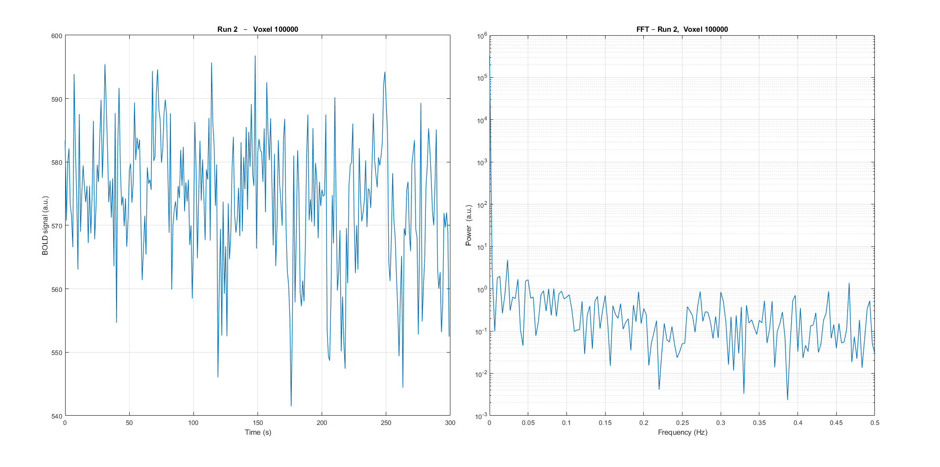
        Plotting the 100kth voxel bold time series and the corresponding Fast Fourier Transform (FFT).

    • a high pass filter at 1/40 Hz is applied, then we can visualise the same voxel data after filtering, notice how the power frequencies lower than 1/40Hz is much smaller

    • convert the bold signals for each voxel to percentage change w.r.t to the average value for that voxel over time, a plot is provided to see the percentage change

      • Example:

        

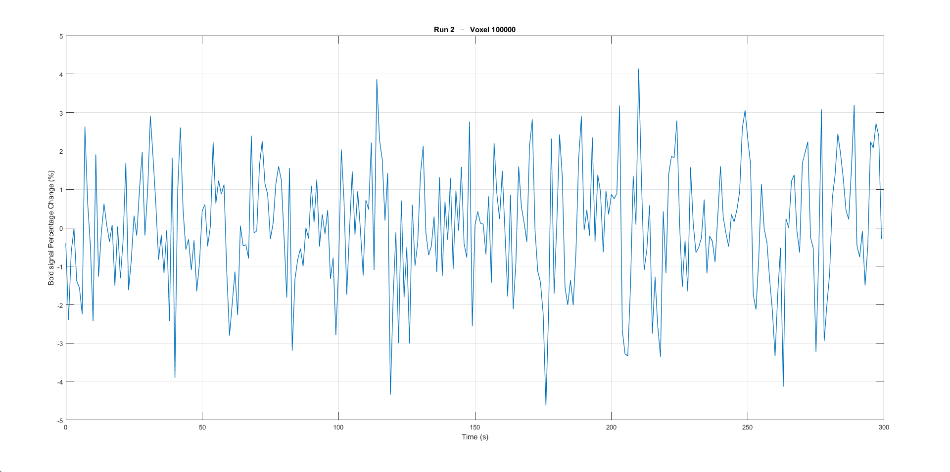
        Plotting the 100kth voxel bold signal percentage change.

• Creating the deisgnMatrix and GLM learning in MATLAB using script in main.m in pipeline/eeg_fmri_pipelines/finger-tapping directory, make sure to open MATLAB from the script itself

  • In the finger-tapping experiment, the participant was asked to tap the same finger for the whole duration of the block (20 seconds), then repeated for other fingers

    • We had randomised the order of the fingers

    • First we are retrieving the order of the fingers that has been stored by the PsychToolBox experiment on NYU BOX

  • Then we will build the designMatrix

    • Build the design matrix with shape (n_TR, n_conditions, n_runs) involving:

      • n_conditions = 13

        • the five conditions for each finger, (finger labelled as 1 is the first column, finger 2)

          • these columns are created as binary mask from the saved matlab random finger tapping output on BoxEEG-FMRIDatafingertappingsub-0665matlab

          • the columns are then convolved with a gamma pdf

        • a drift vector over a run length (1,…,300)

        • a constant vector (1,…,1)

        • 6 motion regressors (trans_x, trans_y, trans_z, rot_x, rot_y, rot_z)

      • n_TR = 300 seconds per run (TR = 1 second)

      • n_runs

        • three runs for the considered session

      • n_voxels = 320721

        • the number of voxels 324k for our case

• Run the GLM

• Save the GLM outputs

• Visually inspect GLM outputs in freeview

• Visualise Betas, use the visualise_betas.sh commands under pipeline/eeg_fmri_pipelines/fmri_preprocessing/finger-tapping

  • the index finger betas are saved as two files in the current directory as lh.betas_index.mgz and ‘rh.betas_index.mgz`

  • to inspect them, run the second command in visualise_betas.sh, you should see the left hemisphere

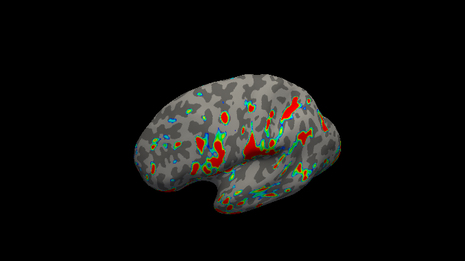
    • within freeview, load the lh.betas_index.mgz by going to Overlay, Load generic and load the file

      • Do not press the Apply Registration when loading the overlay, as we have not changed the space from the brain surface and the overlay, they are both fsnative

      

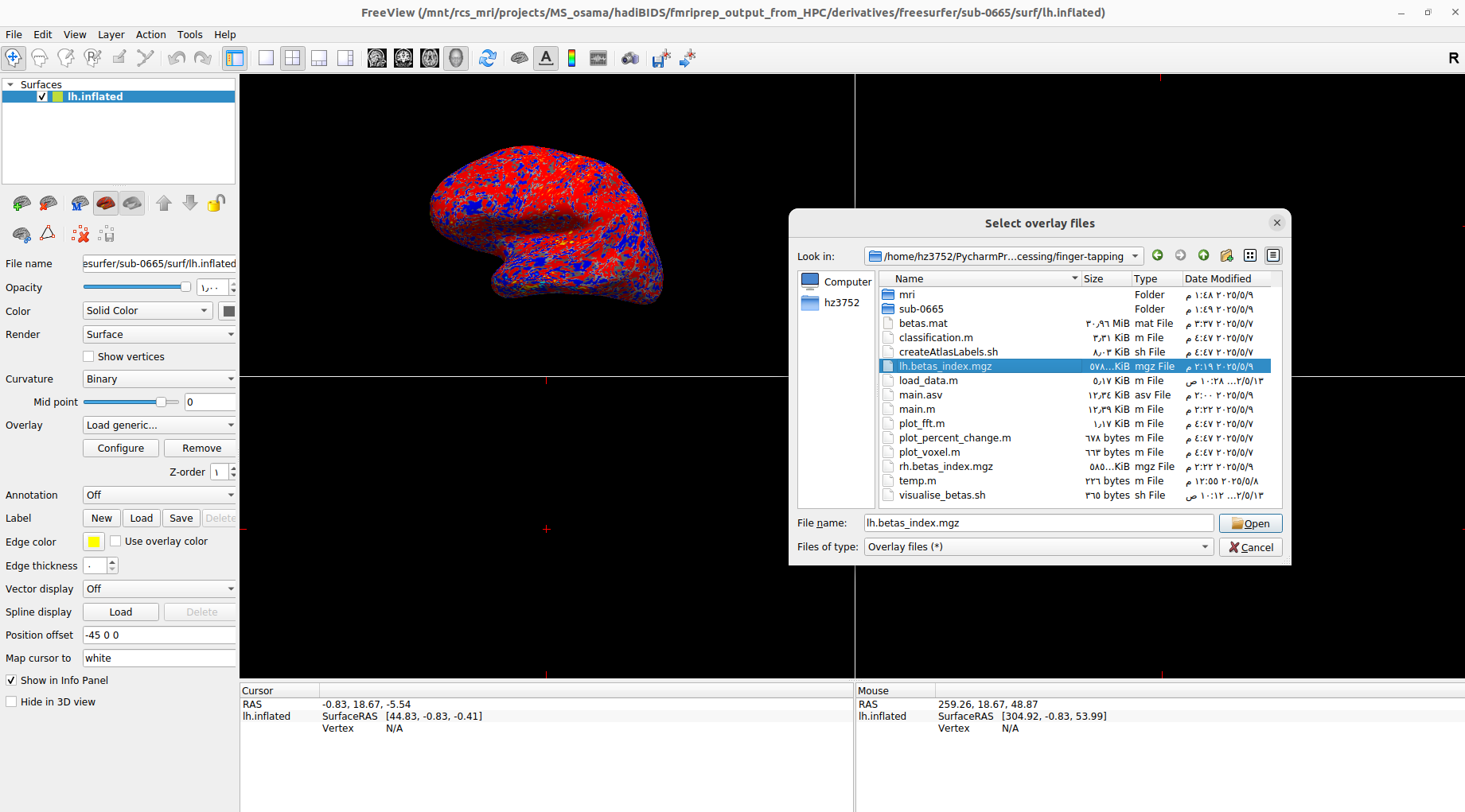
      Loading an overlay of the maximum betas for the index finger on inflated left hemisphere.

  • for the right hemisphere run similar commands on the rh.inflated file

    freeview -f $BIDS_DIR/derivatives/freesurfer/sub-0665/surf/rh.inflated
    

  • press Configure, and adjust the heatmap to show the highest values

    • start with the following parameters for the heatmap configuration and then adjust

      • Use percentile 75 to 90%

      • Enable smooth to 20 steps

      • Color wheel

      • Enable Inverse

  • below are the maximum betas per finger for respectively left and right hemisphere

    

    Thumb finger.

    

    Index finger.

    

    Middle finger.

    

    Ring finger.

    

    Pinkie finger.

Other possible processing steps

These processing steps can enhance your processing pipelines depending on your paradigm.

• Draining vein effect correction (linear offset or CBV scaling or spatial deconvolution)

• Vascular Space Occupancy combined with EEG

• Nordic denoising, with time there is more heating that causes higher amplitudes so this requires denoising

Preparation of the forward/head model

Perform fMRI-informed EEG source reconstruction

• Coregistration requires computing the transformation, use the “layout” file that should help you match the electrodes with the headface

• Some technique uses the ultrasound protocol to locate the electrode and get a geometrical representation of the electrodes

Other methods

• Typical fMRI uses the GLM fitting, with EEG data it is possible to add regressors

  • Proposed method is to take the variability of the EEG data and inject that as regressor into the GLM (variability can be each trial variability or spectral feature such as correlation with a band, or temporal feature ERP peak … this will depend on your paradigm)

  • The non-stimulus activity can be used to correlate baselines (from eeg and fmri) together

Resources and Training Materials

Manuals and Support Teams

Manuals

Manuals can be downloaded from the website: Brain Products Manuals

Technical Support

• Email: techsup@brainproducts.com

• For questions about hardware, recording software, and MR-related artifact handling in Analyzer 2

Analyzer Support

• Email: support@brainproducts.com

• For questions about using Analyzer 2

Support Tips

• Recorder workspace settings for EEG-fMRI: Recorder setup EEG-fMRI

• Best practices: EEG-fMRI Best Practices

• Peripheral physiology measurements using BrainAmp ExG MR: - Part 1: Let’s focus on EMG: EMG-fMRI Guide - Part 2: Let’s focus on ECG: ECG-fMRI Guide

Webinars

Webinar Channels

• Brain Products Webinar Channel

• Brain Products Academy Channel

Analyzer Webinars

• Introduction to Analyzer 2 & EEG analysis concepts: Watch webinar Analyzer 2 EEG

• EEG artifact types and handling strategies in BrainVision Analyzer 2: Watch webinar Artifact Type EEG

EEG-fMRI Webinars

• Joint EEG-fMRI data analysis - Session 1: Introduction to EEG-fMRI: Watch on YouTube - Session 2: EEG-fMRI Data preprocessing and considerations: Watch on YouTube Preprocessing - Session 3: Combining EEG and fMRI data analysis: Watch on YouTube Comining EEG/fMRI

• Handling scanner-related artifacts: Watch webinar artifacts

• CWLs: Watch webinar CWLs

• Getting ready for simultaneous EEG-fMRI: Safety and setup basics: Watch webinar Basic Setup

Keep Up to Date

Sign up for the newsletter to receive information on events, support tips, and new products: Subscribe here